Systems of partial differential equations and Lie by J. Pommaret
By J. Pommaret
Read Online or Download Systems of partial differential equations and Lie pseudogroups PDF
Best differential equations books
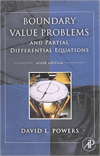
Boundary Value Problems: And Partial Differential Equations
Boundary price difficulties is the best textual content on boundary worth difficulties and Fourier sequence for pros and scholars in engineering, technological know-how, and arithmetic who paintings with partial differential equations. during this up-to-date version, writer David Powers presents an intensive evaluate of fixing boundary worth difficulties related to partial differential equations via the tools of separation of variables.

Invertible Point Transformations and Nonlinear Differential Equations
The invertible aspect transformation is a robust device within the learn of nonlinear differential and distinction questions. This ebook supplies a entire creation to this method. usual and partial differential equations are studied with this method. The e-book additionally covers nonlinear distinction equations.
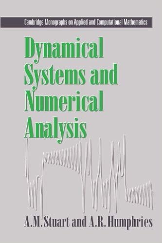
Dynamical systems and numerical analysis
This e-book unites the learn of dynamical structures and numerical answer of differential equations. the 1st 3 chapters comprise the weather of the idea of dynamical platforms and the numerical resolution of initial-value difficulties. within the closing chapters, numerical equipment are formulted as dynamical platforms and the convergence and balance homes of the tools are tested.
- Domain Decomposition Methods for Partial Differential Equations (Numerical Mathematics and Scientific Computation)
- Volterra Integral and Differential Equations, Edition: 2nd ed
- Partial Differential Equations
- An Introduction to Ordinary Differential Equations (Dover Books on Mathematics)
- Introduction to Partial Differential Equations for Scientists and Engineers Using Mathematica
Extra resources for Systems of partial differential equations and Lie pseudogroups
Example text
14) ¯ 2 M# 0 (Ω, R ), Aµ,Ω = sup ¯ Ω L2 (Ω) ≤ √ L2 (Ω) 2 ∇ϕ L2 (Ω) . 14) is achieved by some unique ϕ ∈ H1 (Ω; R2 ) modulo ¯ R2 ) by Theorem 2 in [5] (when µ is an L1 constants; moreover, ϕ ∈ (L∞ ∩ C)(Ω; function — the case of measures is similar). ¯ 2 Thus we have for every µ ∈ M# 0 (Ω, R ) µ . 15) ¯ 2 AΩ = sup Aµ,Ω : µ ∈ M# 0 (Ω, R ) and µ ≤ 1 . 10. One has 1 1 √ < AΩ ≤ √ . 15) is achieved. Proof. Let µ = λt H1 ∂B(x0 , r) with ∂B(x0 , r) ⊂ Ω and (x − x0 )⊥ r2 (x − x0 )⊥ |x−x 2 0| ϕ(x) = if |x − x0 | ≤ r , if |x − x0 | > r .
GP] D. Girela, J. A. Pel´ aez, Boundary behaviour of analytic functions in spaces of Dirichlet type, J. Inequal. Appl. 2006, Art. ID 92795, 12 pp. [KV] N. Kalton, I. Verbitsky. Nonlinear equations and weighted norm inequalities, Trans. Amer. Math. Soc. 351 (1999), no. 9, 3441–3497. odinger op[KS] R. Sawyer, The trace inequality and eigenvalue estimates for Schr¨ erators, Ann. Inst. Fourier (Grenoble) 36 (1986), no. 4, 207–228. [Ki] J. Kinney, Tangential limits of functions of the class Sα , Proc.
Thus DF (3) ∈ l2 (T, 2−εd(α) ). We now use the same arguments as before. Set G = I(DF (3) ); G will have finite radial limits along every geodesic Γ with the possible exception of a set which is a null set for every Carleson measure for the space Dd,ε . Also as in the previous proof, any boundary point Γ at which I(DF (3) )(Γ) < ∞ will be a boundary point where we have good convergence of F ; in this case the good convergence meaning convergence over Γ3 (ε). The description of the Carleson measures for these spaces is given in [AR].