Invertible Point Transformations and Nonlinear Differential by Steeb W.-H.
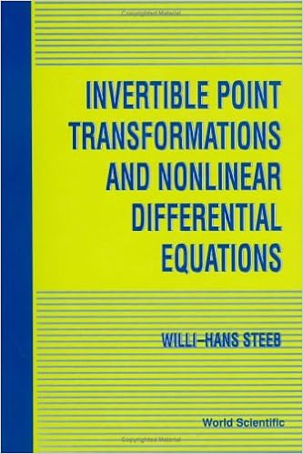
By Steeb W.-H.
The invertible element transformation is a robust software within the research of nonlinear differential and distinction questions. This publication offers a complete creation to this method. traditional and partial differential equations are studied with this process. The publication additionally covers nonlinear distinction equations. The connections with Lie symmetries, the Painleve estate, first integrals and the Cartan equivalence technique are mentioned intimately. many of the reviews are checked with the pc language decrease; the e-book contains 30 decrease courses. a brief advent to the jet package formalism is given
Read Online or Download Invertible Point Transformations and Nonlinear Differential Equations PDF
Best differential equations books
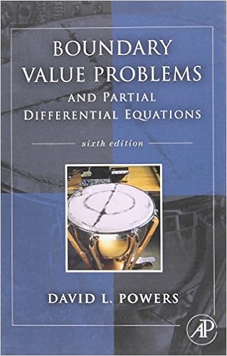
Boundary Value Problems: And Partial Differential Equations
Boundary worth difficulties is the top textual content on boundary price difficulties and Fourier sequence for execs and scholars in engineering, technology, and arithmetic who paintings with partial differential equations. during this up to date version, writer David Powers offers a radical evaluation of fixing boundary price difficulties regarding partial differential equations via the tools of separation of variables.

Invertible Point Transformations and Nonlinear Differential Equations
The invertible element transformation is a robust device within the examine of nonlinear differential and distinction questions. This publication supplies a entire creation to this system. traditional and partial differential equations are studied with this procedure. The e-book additionally covers nonlinear distinction equations.
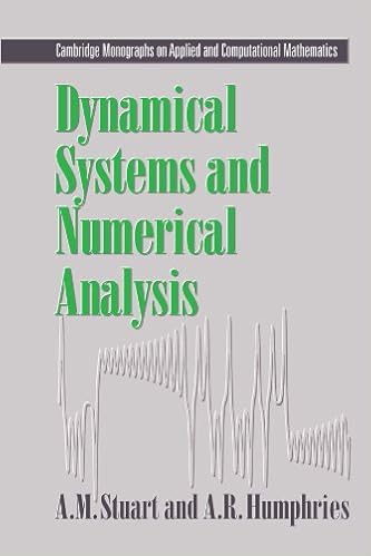
Dynamical systems and numerical analysis
This booklet unites the learn of dynamical structures and numerical resolution of differential equations. the 1st 3 chapters comprise the weather of the speculation of dynamical platforms and the numerical answer of initial-value difficulties. within the final chapters, numerical tools are formulted as dynamical structures and the convergence and balance houses of the tools are tested.
- A Minicourse on Stochastic Partial Differential Equations (Lecture Notes in Mathematics)
- Nonlinear Diffusion Equations
- Methods on Nonlinear Elliptic Equations (Aims Series on Differential Equations & Dynamical Systems)
- Fourier Series and Boundary Value Problems
Extra info for Invertible Point Transformations and Nonlinear Differential Equations
Sample text
Physics Formulary by ir. A. 10 Spin For the spin operators are defined by their commutation relations: [S x , Sy ] = i¯ hSz . Because the spin operators do not act in the physical space (x, y, z) the uniqueness of the wavefunction is not a criterium here: also half odd-integer values are allowed for the spin. Because [L, S] = 0 spin and angular momentum operators do not ¯ σ, with have a common set of eigenfunctions. The spin operators are given by S = 12 h σx = 0 1 1 0 , σy = 0 −i i 0 1 0 0 −1 , σz = The eigenstates of Sz are called spinors: χ = α+ χ+ + α− χ− , where χ+ = (1, 0) represents the state with spin up (Sz = 12 h ¯ ) and χ− = (0, 1) represents the state with spin down (Sz = − 12 h ¯ ).
If Pr 1: δ/δT ≈ 3 Pr. 8 Heat conductance For non-stationairy heat conductance in one dimension without flow holds: κ ∂2T ∂T = +Φ ∂t c ∂x2 where Φ is a source term. If Φ = 0 the solutions for harmonic oscillations at x = 0 are: T − T∞ x x = exp − cos ωt − Tmax − T∞ D D Physics Formulary by ir. A. Wevers 44 with D = 2κ/ω c. At x = πD the temperature variation is in anti-phase with the surface. The onedimensional solution at Φ = 0 is 1 x2 T (x, t) = √ exp − 4at 2 πat This is mathematical equivalent to the diffusion problem: ∂n = D∇2 n + P − A ∂t where P is the production of and A the discharge of particles.
5 Waveguides and resonating cavities The boundary conditions for a perfect conductor can be derived from the Maxwell equations. If n is a unit vector ⊥ the surface, pointed from 1 to 2, and K is a surface current density, than holds: n · ( D2 − D1 ) = σ n · ( B2 − B1 ) = 0 n × ( E2 − E1 ) = 0 n × ( H2 − H1 ) = K In a waveguide holds because of the cylindrical symmetry: E(x, t) = E(x, y)ei(kz−ωt) and B(x, t) = B(x, y)ei(kz−ωt) . From this one can now deduce that, if Bz and Ez are not ≡ 0: ∂Ez i ∂Bz − εµω k εµω 2 − k 2 ∂x ∂y ∂Bz i ∂Ez + εµω Ex = k εµω 2 − k 2 ∂x ∂y Bx = ∂Ez i ∂Bz + εµω k εµω 2 − k 2 ∂y ∂x ∂Bz i ∂Ez − εµω Ey = k εµω 2 − k 2 ∂y ∂x By = Now one can distinguish between three cases: 1.