Homogenization : Methods and Applications by G. A. Chechkin
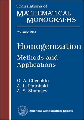
By G. A. Chechkin
Homogenization is a suite of strong thoughts in partial differential equations which are used to check differential operators with quickly oscillating coefficients, boundary worth issues of swiftly various boundary stipulations, equations in perforated domain names, equations with random coefficients, and different gadgets of theoretical and useful curiosity. The publication makes a speciality of a variety of features of homogenization idea and comparable subject matters. It includes classical effects and strategies of homogenization idea, in addition to glossy matters and strategies constructed within the final decade. unique consciousness is paid to averaging of random parabolic equations with reduce order phrases, to homogenization of singular buildings and measures, and to issues of speedily alternating boundary stipulations. The ebook comprises many routines, which aid the reader to higher comprehend the cloth offered. all of the major effects are illustrated with numerous examples, starting from extremely simple to fairly complicated.
Read or Download Homogenization : Methods and Applications PDF
Best differential equations books
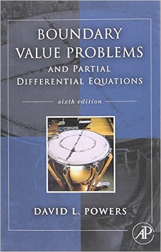
Boundary Value Problems: And Partial Differential Equations
Boundary price difficulties is the best textual content on boundary price difficulties and Fourier sequence for pros and scholars in engineering, technology, and arithmetic who paintings with partial differential equations. during this up to date version, writer David Powers offers an intensive review of fixing boundary worth difficulties related to partial differential equations via the tools of separation of variables.
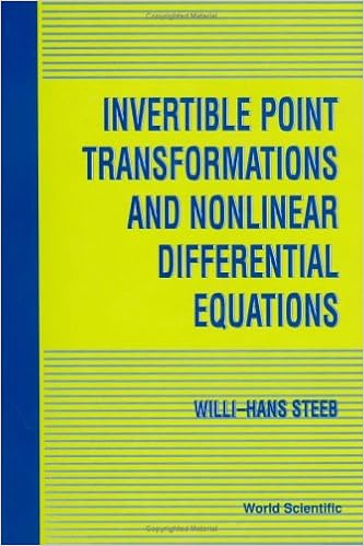
Invertible Point Transformations and Nonlinear Differential Equations
The invertible element transformation is a robust software within the examine of nonlinear differential and distinction questions. This publication offers a finished creation to this method. usual and partial differential equations are studied with this method. The booklet additionally covers nonlinear distinction equations.
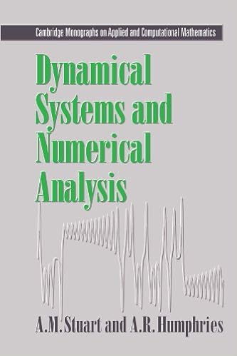
Dynamical systems and numerical analysis
This publication unites the research of dynamical platforms and numerical resolution of differential equations. the 1st 3 chapters include the weather of the idea of dynamical platforms and the numerical answer of initial-value difficulties. within the final chapters, numerical equipment are formulted as dynamical platforms and the convergence and balance houses of the tools are tested.
- Polyharmonic boundary value problems
- Linear Differential Equations With Periodic Coefficients, volume 1
- Nonlinear Singular Perturbation Phenomena: Theory and Applications (Applied Mathematical Sciences)
- Laplace-transformation Fur ingenieure Der Elektrotechnik
Additional info for Homogenization : Methods and Applications
Sample text
184) Set C0 J0 , E := y ∈ C J0 , E : y(0) = a . e. e. e. t ∈ J0 , A1 = t ∈ J : y(t) < y(t) ≤ y(t) , A2 = t ∈ J : y(t) ≤ y(t) < y(t) . 27. For each y ∈ C(J, E), the set S1F,τ y is nonempty. 1), there exists v ∈ S1F,y . 188) A3 = t ∈ J : y(t) ≤ y(t) ≤ y(t) . 189) where Then by decomposability w ∈ S1F,τ y . 7. Claim 1. G(y) is convex for each y ∈ C0 (J0 , E). This is obvious since S1F,τ y is convex (because F has convex values). Claim 2. G sends bounded sets into relatively compact sets in C0 (J0 , E).
Then for each h ∈ G(y) there exists v ∈ S1F,y such that t h(t) = T(t)a + 0 T(t − s)v(s)ds, t ∈ J0 . 152) . Claim 3. G sends bounded sets in C(J0 , E) into equicontinuous sets. Let u1 , u2 ∈ J0 , u1 < u2 , Br := { y ∈ C(J0 , E) : y ∞ ≤ r } be a bounded set in C0 (J0 , E) as in Claim 2 and y ∈ Br . 153) ≤ T u2 a − T u1 a u2 + 0 T u2 − s − T u1 − s v(s)ds u2 +M v(s) ds. 3), together with the Arzel´a-Ascoli theorem, we can conclude that G : C(J0 , E) → P (C(J0 , E)) is a compact multivalued map, and therefore, a condensing map.
92) i = 0, . . , m − 1. 93) f t, ri (t) dt ≤ ri wi − ri zi , i = 0, . . , m with zi < w i , zi , wi ∈ ti , ti+1 . 54) has at least one solution. e. t ∈ J, t = tk , k = 1, . . , m, Δy |t=tk = Ik y tk− , k = 1, . . 95) y(0) = y0 , where F : J × Rn → P (Rn ) is a multivalued map with nonempty compact values, y0 ∈ Rn , P (Rn ) is the family of all subsets of Rn , Ik ∈ C(Rn , Rn ) (k = 1, 2, . . , m), Δy |t=tk = y(tk+ ) − y(tk− ), y(tk− ) and y(tk+ ) represent the left and right limits of y(t) at t = tk , respectively.