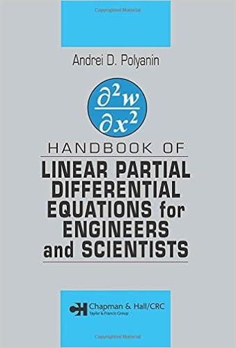
Handbook of Linear Partial Differential Equations for by Andrei D. Polyanin
By Andrei D. Polyanin
Following within the footsteps of the authors' bestselling instruction manual of necessary Equations and instruction manual of tangible recommendations for usual Differential Equations, this instruction manual offers short formulations and targeted ideas for greater than 2,200 equations and difficulties in technology and engineering."Parabolic, hyperbolic, and elliptic equations with consistent and variable coefficients"New particular ideas to linear equations and boundary worth problems"Equations and difficulties of common shape that rely on arbitrary functions"Formulas for developing suggestions to nonhomogeneous boundary price problems"Second- and higher-order equations and boundary price problemsAn introductory part outlines the elemental definitions, equations, difficulties, and strategies of mathematical physics. It additionally presents invaluable formulation for expressing strategies to boundary price difficulties of normal shape by way of the Green's functionality. vitamins on the finish of the e-book provide extra instruments and data: complement A lists the homes of universal distinct capabilities, together with the gamma, Bessel, degenerate hypergeometric, and Mathieu features, and complement B describes the equipment of generalized and practical separation of variables for nonlinear partial differential equations.
Read or Download Handbook of Linear Partial Differential Equations for Engineers and Scientists PDF
Similar differential equations books
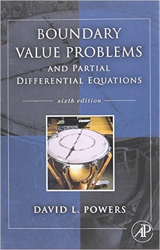
Boundary Value Problems: And Partial Differential Equations
Boundary worth difficulties is the major textual content on boundary price difficulties and Fourier sequence for execs and scholars in engineering, technology, and arithmetic who paintings with partial differential equations. during this up-to-date variation, writer David Powers offers a radical evaluate of fixing boundary worth difficulties related to partial differential equations by means of the tools of separation of variables.

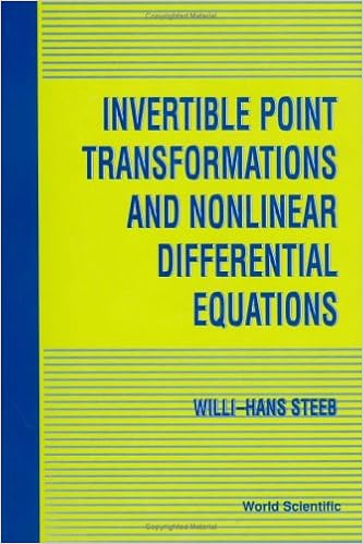
Invertible Point Transformations and Nonlinear Differential Equations
The invertible element transformation is a strong device within the examine of nonlinear differential and distinction questions. This ebook offers a entire creation to this system. traditional and partial differential equations are studied with this technique. The publication additionally covers nonlinear distinction equations.
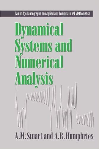
Dynamical systems and numerical analysis
This e-book unites the research of dynamical structures and numerical resolution of differential equations. the 1st 3 chapters include the weather of the idea of dynamical structures and the numerical resolution of initial-value difficulties. within the final chapters, numerical tools are formulted as dynamical platforms and the convergence and balance homes of the tools are tested.
- Modelling with Differential and Difference Equations (Australian Mathematical Society Lecture Series)
- Theory of functional differential equations, Edition: 2d ed
- Handbook of first order partial differential equations
- Approximate Analytical Methods for Solving Ordinary Differential Equations
- Applied partial differential equations. An introduction
- Asymptotic Expansions for Ordinary Differential Equations
Extra info for Handbook of Linear Partial Differential Equations for Engineers and Scientists
Example text
Solution: ✄ ✂ ü ( , )= û ÿ û ☎ û ) ✠ ☞ ✌ 1) þ 1( ✡ sin ☎ þ ☎ ✝ ✞ + ☎ 2 û , − ) û ✝ ✞ ( − 2− û ✜ ✑ ✏ =1 ☛ ✠ þ ( , ) ( , , − ) ù 0 ✄ − ✠ 2( 0 sin 1 þ ✠ ) ✠ , )= û ( , , ) ✆ û ☎ ✝ ✓ = ✓ ☎ ✘✚✙ ☎ ✝ 2( ✡ ✑ ( − 2− ✏ þ ✢ , − ) û ✝ ✠ 1) þ 1 ≤ ≤ û ☎ ✞ ✞ ✠ , ✠ 2 2 ( ✜ 1 þ ✢ , ✄ 2( ✡ 1 , )= û ý ✝ ( , , ) ✆ û ☎ ✝ 2. þ ✓ = ✓ ☎ 2− ✑ ✏ þ þ ➾ , ✝ 1) 2 ✢ . ✄ 2 ✓✣✔ Reference: H. S. Carslaw and J. C. Jaeger (1984). 4-5. Domain: ✠ ý ý ✝ û ☎ ✜ ý 1( ✡ ✆ ✟ ➾ 1) þ ☎ 1 ✂ 1( 0 2 ( 2− ✝ ✆ ✄ ✂ ✟ ➾ where ( , , )= ☎ 1 ✂ + ✆ ( ) ( , , ) ✝ ✄ ✟ ✂ 2 Second boundary value problem.
Solution: ✄ ✂ ü ( , )= û ( ) ( , , ) ÿ ☎ 0 ✆ û ☎ Here, ✝ ✞ + ☎ ( ) ( , , − ) ✠ 0 2 ( , , )= û ✌ ☎ ✆ û þ ✝ ✠ ✛ þ where the û ☛ 2 =1 + ✠ ✛ þ ✛ ✎ þ þ ✗ ( , ) ( , , − ) ù sin û þ ✄ ✂ 0 ✌ +( − 1)2 sin + ( − 1) ☞✍✌ ☎ ✝ ✞ 2 ✌ ✟ ✂ ➾ ✌ ✆ ✘✚✙ ✟ ✂ ✝ ☎ 0 ✠ ✆ û ☎ ✌ 2 exp − ☎ ➾ þ ✒ þ ✗ ✗ ☎ ✞ ✠ . ✒ ✗ cot + are positive roots of the transcendental equation ✞ , ✝ 2 ✎ ✗ ✠ ✌ ✎ ✒ ✝ ✛ − 1 = 0. þ Reference: H. S. Carslaw and J. C. Jaeger (1984). 4-4. Domain: ≤ 1 þ ≤ û 2. þ ✗ First boundary value problem. The following conditions are prescribed: = ( ) at = 1 ( ) at ü ÿ ü û = ü ✝ ✝ 2( û ) at ✝ =0 = þ 1 (initial condition), (boundary condition), = þ 2 (boundary condition).
3-10. Domain: 0 ≤ ❾ ≤ ◗ . Mixed boundary value problem. The following conditions are➁ prescribed: ➁ = ➀ (❾ ) ➐ ➁ ❸ Solution: ➐ = ➌ 1 ( ) at ➐ = ➌ 2 ( ) at ➔ =0 at (initial condition), = 0 (boundary condition), = ◗ (boundary condition). ❾ ❾ ➁ ❻ ➐ (❾ , ) = ➂ (❼ ) (❾ , ❼ , ) ➄ ❘ ➀ 0 + ❻ ➐ ➈ 0 ➅ ➂ 0 + ➆ ➐ (❼ , ➆ ) (❾ , ❼ , − ➆ ) ➄ ❘ ❹ 0 ➐ ) ➢ (❾ , − ➆ ) ➄ 1 (➆ ➅ ➌ ➂ +➂ ❼ ❻ ➈ ➅ ➌ ➂ 0 ❼ ➐ ) (❾ , ◗ , − ➆ ) ➄ 2 (➆ ➄ ➆ ➆ , where ❻ ➐ (❾ , ❼ , ) = 2 sin ➉ ➃ ❽ ➎ ◗ ➅ =0 ❻ ❸ ➐ (❾ , ) = ➢ ⑩ ➣↔ ➐ (❾ , ❼ , ) ➛ ❸ ➛ ❼ ➛❨➜ ⑩ (2 + 1)❾ ➙ 2◗ =0 sin ➉ ➊ ➈ ⑩ (2 + 1)❼ ➙ 2◗ exp ➉ − ➊ 2 (2 + 1)2 ➙ 4◗ 2 ➐ ➊ , .