Schaum's Easy Outline: Differential Equations (Schaum's by Richard Bronson

By Richard Bronson
Boiled-down necessities of the top-selling Schaum's define sequence, for the scholar with constrained time What will be greater than the bestselling Schaum's define sequence? for college kids searching for a brief nuts-and-bolts review, it can must be Schaum's effortless define sequence. each e-book during this sequence is a pared-down, simplified, and tightly targeted model of its greater predecessor. With an emphasis on readability and brevity, each one new identify contains a streamlined and up-to-date structure and absolutely the essence of the topic, awarded in a concise and quite simply comprehensible shape. photo components equivalent to sidebars, reader-alert icons, and boxed highlights characteristic chosen issues from the textual content, remove darkness from keys to studying, and provides scholars quickly tips to the necessities.
Read or Download Schaum's Easy Outline: Differential Equations (Schaum's Outline Series) PDF
Best differential equations books
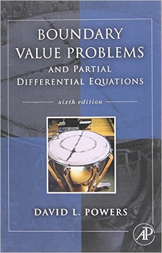
Boundary Value Problems: And Partial Differential Equations
Boundary worth difficulties is the best textual content on boundary price difficulties and Fourier sequence for pros and scholars in engineering, technology, and arithmetic who paintings with partial differential equations. during this up-to-date version, writer David Powers offers an intensive assessment of fixing boundary price difficulties concerning partial differential equations by means of the tools of separation of variables.
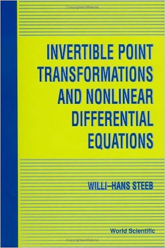
Invertible Point Transformations and Nonlinear Differential Equations
The invertible element transformation is a strong device within the research of nonlinear differential and distinction questions. This booklet provides a finished advent to this system. traditional and partial differential equations are studied with this procedure. The publication additionally covers nonlinear distinction equations.
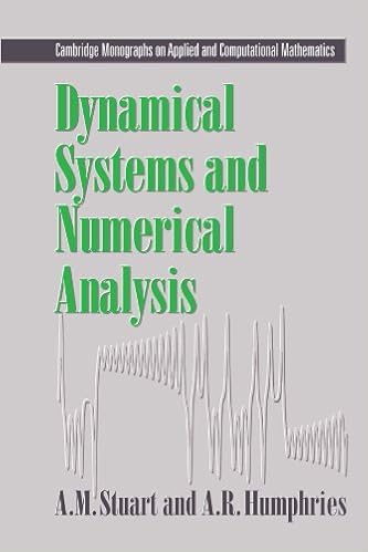
Dynamical systems and numerical analysis
This e-book unites the examine of dynamical structures and numerical answer of differential equations. the 1st 3 chapters include the weather of the speculation of dynamical platforms and the numerical resolution of initial-value difficulties. within the ultimate chapters, numerical equipment are formulted as dynamical platforms and the convergence and balance houses of the equipment are tested.
- Integral Dynamical Models : Singularities, Signals and Control (World Scientific Series on Nonlinear Science Series a)
- Linear and Nonlinear Parabolic Complex Equations
- Solving Nonlinear Equations with Newton's Method (Fundamentals of Algorithms)
- Partial Differential Equations (Proceedings of Symposia in Pure Mathematics, vol. 4)
- Reconstruction of Small Inhomogeneities from Boundary Measurements (Lecture Notes in Mathematics)
Additional resources for Schaum's Easy Outline: Differential Equations (Schaum's Outline Series)
Sample text
If this limit does not exist, the improper integral diverges and f(x) has no Laplace transform. 1, the variable s is treated as a constant because the integration is with respect to x. The Laplace transforms for a number of elementary functions are given in Appendix A. 1 (Linearity). 2. 3. 4. 5. 6. 8, are presented for functions of x. They are equally applicable for functions of any independent variable and are generated by replacing the variable x in the above equations by any variable of interest.
8m/sec2, we have w = mg = 98 N and k = w/l = 140 N/m. Furthermore, a = 90 and F(t) ≡ 0 (there is no external force). 14) The roots of the associated characteristic equation are l1 = −2 and l2 = −7, which are real and distinct; hence this problem is an example of overdamped motion. 14 is x = c1e −2 t + c2 e −7t The initial conditions are x(0) = 0 (the mass starts at the equilibrium position) and x˙(0) = −1 (the initial velocity is in the negative direction). Applying these conditions, we find that c1 = − c2 = − 15 , so that x = −7t 1 5 (e − e −2 t ).
These arbitrary constants are then evaluated by substituting the proposed solution into the given differential equation and equating the coefficients of like terms. Case 1. f(x) = pn(x), an nth-degree polynomial in x. , n) is a constant to be determined. Case 2. f(x) = keax where k and a are known constants. 2) where A is a constant to be determined. Case 3. f(x) = k1 sin bx + k2 cos bx where k1, k2, and b are known constants. Assume a solution of the form yp = A sin bx + B cos bx where A and B are constants to be determined.