Numerische Behandlung nichtlinearer Integrodifferential- und by R. Ansorge, W. Törnig
By R. Ansorge, W. Törnig
Read or Download Numerische Behandlung nichtlinearer Integrodifferential- und Differentialgleichungen PDF
Similar differential equations books
Boundary Value Problems: And Partial Differential Equations
Boundary worth difficulties is the major textual content on boundary worth difficulties and Fourier sequence for pros and scholars in engineering, technology, and arithmetic who paintings with partial differential equations. during this up to date variation, writer David Powers presents an intensive review of fixing boundary worth difficulties regarding partial differential equations via the tools of separation of variables.
Invertible Point Transformations and Nonlinear Differential Equations
The invertible element transformation is a strong instrument within the research of nonlinear differential and distinction questions. This booklet provides a complete advent to this system. usual and partial differential equations are studied with this technique. The booklet additionally covers nonlinear distinction equations.
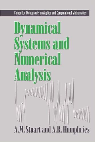
Dynamical systems and numerical analysis
This e-book unites the examine of dynamical platforms and numerical answer of differential equations. the 1st 3 chapters comprise the weather of the speculation of dynamical platforms and the numerical answer of initial-value difficulties. within the ultimate chapters, numerical tools are formulted as dynamical structures and the convergence and balance homes of the tools are tested.
- Guide to Distribution Theory and Fourier
- Stochastic Parameterizing Manifolds and Non-Markovian Reduced Equations: Stochastic Manifolds for Nonlinear SPDEs II (SpringerBriefs in Mathematics)
- Partial Differential Equations. Qualitative studies of linear equations
- Elementary Differential Equations And Boundary Value Problems - Boyce And Diprima Student Solutions Manual, Edition: 7th
- Elliptic and Parabolic Equations: Hannover, September 2013 (Springer Proceedings in Mathematics & Statistics)
Additional resources for Numerische Behandlung nichtlinearer Integrodifferential- und Differentialgleichungen
Example text
184) Set C0 J0 , E := y ∈ C J0 , E : y(0) = a . e. e. e. t ∈ J0 , A1 = t ∈ J : y(t) < y(t) ≤ y(t) , A2 = t ∈ J : y(t) ≤ y(t) < y(t) . 27. For each y ∈ C(J, E), the set S1F,τ y is nonempty. 1), there exists v ∈ S1F,y . 188) A3 = t ∈ J : y(t) ≤ y(t) ≤ y(t) . 189) where Then by decomposability w ∈ S1F,τ y . 7. Claim 1. G(y) is convex for each y ∈ C0 (J0 , E). This is obvious since S1F,τ y is convex (because F has convex values). Claim 2. G sends bounded sets into relatively compact sets in C0 (J0 , E).
Then for each h ∈ G(y) there exists v ∈ S1F,y such that t h(t) = T(t)a + 0 T(t − s)v(s)ds, t ∈ J0 . 152) . Claim 3. G sends bounded sets in C(J0 , E) into equicontinuous sets. Let u1 , u2 ∈ J0 , u1 < u2 , Br := { y ∈ C(J0 , E) : y ∞ ≤ r } be a bounded set in C0 (J0 , E) as in Claim 2 and y ∈ Br . 153) ≤ T u2 a − T u1 a u2 + 0 T u2 − s − T u1 − s v(s)ds u2 +M v(s) ds. 3), together with the Arzel´a-Ascoli theorem, we can conclude that G : C(J0 , E) → P (C(J0 , E)) is a compact multivalued map, and therefore, a condensing map.
92) i = 0, . . , m − 1. 93) f t, ri (t) dt ≤ ri wi − ri zi , i = 0, . . , m with zi < w i , zi , wi ∈ ti , ti+1 . 54) has at least one solution. e. t ∈ J, t = tk , k = 1, . . , m, Δy |t=tk = Ik y tk− , k = 1, . . 95) y(0) = y0 , where F : J × Rn → P (Rn ) is a multivalued map with nonempty compact values, y0 ∈ Rn , P (Rn ) is the family of all subsets of Rn , Ik ∈ C(Rn , Rn ) (k = 1, 2, . . , m), Δy |t=tk = y(tk+ ) − y(tk− ), y(tk− ) and y(tk+ ) represent the left and right limits of y(t) at t = tk , respectively.