Numerical Solution of Partial Differential Equations by the by Claes Johnson
By Claes Johnson
An available advent to the finite aspect strategy for fixing numeric difficulties, this quantity bargains the keys to a huge procedure in computational arithmetic. appropriate for complicated undergraduate and graduate classes, it outlines transparent connections with functions and considers a number of examples from quite a few technological know-how- and engineering-related specialties. 1987 edition.
Bibliographical Note
This Dover variation, first released in 2009, is an unabridged republication of the paintings initially released in 1987 via Cambridge collage Press, Cambridge, and Studentlitteratur, Lund, Sweden. the writer has supplied a brand new preface for this version.
Read or Download Numerical Solution of Partial Differential Equations by the Finite Element Method PDF
Similar differential equations books
Boundary Value Problems: And Partial Differential Equations
Boundary price difficulties is the best textual content on boundary worth difficulties and Fourier sequence for pros and scholars in engineering, technology, and arithmetic who paintings with partial differential equations. during this up-to-date variation, writer David Powers presents an intensive evaluation of fixing boundary price difficulties regarding partial differential equations by way of the tools of separation of variables.
Invertible Point Transformations and Nonlinear Differential Equations
The invertible aspect transformation is a robust instrument within the examine of nonlinear differential and distinction questions. This booklet provides a finished advent to this method. usual and partial differential equations are studied with this method. The ebook additionally covers nonlinear distinction equations.
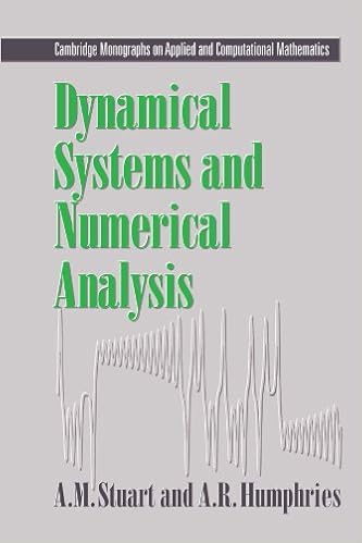
Dynamical systems and numerical analysis
This publication unites the learn of dynamical structures and numerical answer of differential equations. the 1st 3 chapters include the weather of the speculation of dynamical structures and the numerical answer of initial-value difficulties. within the last chapters, numerical tools are formulted as dynamical structures and the convergence and balance houses of the tools are tested.
- Fuchsian Differential Equations: With Special Emphasis on the Gauss-Schwarz Theory (Aspects of Mathematics) (German Edition)
- Partial Differential Equations 1: Foundations and Integral Representations (2nd Edition) (Universitext)
- Lectures on algebraic solutions of hypergeometric differential equations (Lectures in mathematics)
- Complex Analysis and Differential Equations (Springer Undergraduate Mathematics Series)
Additional resources for Numerical Solution of Partial Differential Equations by the Finite Element Method
Sample text
For is = l:delr(l) ist = is; 7. 7o Build the perturbation vector. 7. pt = zeros(n,l); while ist <= n pt(ist) = 1; ist = delr(ist)+l; end 7. 7» Compute the forward difference. 7. xl = x+epsnew*pt; fl = feval(f,xl); dv = (fl-fO)/epsnew; ist = is; 7. % Fill the appropriate columns of the Jacobian. 7. 4. The Chord and Shamanskii Methods 33 The internal MATLAB code numjac is a more general finite difference Jacobian code, numjac was designed to work with the stiff ordinary differential equation integrators [68] in MATLAB.
The components of parms are maxit is the upper limit on the nonlinear iteration; the default is 40, which is usually enough. The Jacobian is computed and factored after every isham nonlinear iterations or whenever the ratio of successive norms of the nonlinear residual is larger than rsham. So, for example, isham — 1 and rsham = 0 is Newton's method. 5, so the Jacobian is updated only if the decrease in the nonlinear residual is not sufficiently rapid. 1) of using an out-of-date Jacobian when far from a solution is reduced.
L; nx=63; nt=l+l/dt; dx=l/(nx+l); tval=0:dt:1; xval=0:dx:1; 7. 7. Use tight tolerances, Newton's method, and a tridiagonal Jacobian. y. d-6]; parms=[40, 1, 0, 1, 1, 1]; uhist=zeros(nx+2,nt); uold=zeros(nx,1); for it=l:nt-l [unew, it_hist, ierr] =nsold (uold,' f time', tol, parms) ; uhist(2:nx+1,it+1)=unew; uold=unew; end 7, 7. Plot the results. 7. 4. 13). 50 Chapter 2. Finding the Newton Step with Gaussian Elimination You can see from the plot that u(x, t) tends to a limit as t —> oo. 14) would be to solve the time-dependent problem and look for convergence of u as t —> oo.