Numerical Solution of Partial Differential Equations: An by K. W. Morton
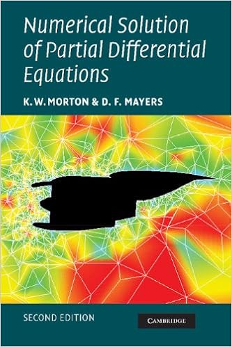
By K. W. Morton
This moment version of a hugely winning graduate textual content offers an entire creation to partial differential equations and numerical research. Revised to incorporate new sections on finite quantity equipment, changed equation research, and multigrid and conjugate gradient tools, the second one version brings the reader updated with the newest theoretical and business advancements. First version Hb (1995): 0-521-41855-0 First variation Pb (1995): 0-521-42922-6
Read Online or Download Numerical Solution of Partial Differential Equations: An Introduction PDF
Best differential equations books
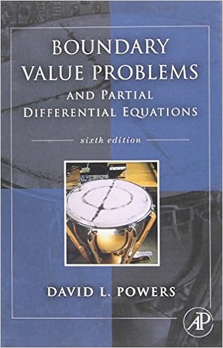
Boundary Value Problems: And Partial Differential Equations
Boundary worth difficulties is the top textual content on boundary price difficulties and Fourier sequence for execs and scholars in engineering, technology, and arithmetic who paintings with partial differential equations. during this up-to-date version, writer David Powers offers a radical evaluate of fixing boundary price difficulties concerning partial differential equations via the tools of separation of variables.
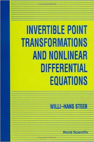
Invertible Point Transformations and Nonlinear Differential Equations
The invertible element transformation is a robust instrument within the learn of nonlinear differential and distinction questions. This publication offers a entire advent to this system. traditional and partial differential equations are studied with this strategy. The publication additionally covers nonlinear distinction equations.
Dynamical systems and numerical analysis
This e-book unites the examine of dynamical platforms and numerical answer of differential equations. the 1st 3 chapters include the weather of the idea of dynamical structures and the numerical resolution of initial-value difficulties. within the ultimate chapters, numerical equipment are formulted as dynamical platforms and the convergence and balance houses of the tools are tested.
- Ordinary Differential Equations: A Brief Eclectic Tour (Classroom Resource Materials)
- The Mollification Method and the Numerical Solution of Ill-Posed Problems
- Tube domains and the Cauchy problem (Translations of Mathematical Monographs)
- Analisi Matematica I: Teoria ed esercizi con complementi in rete (UNITEXT / La Matematica per il 3+2) (Italian Edition)
- Theory of Fuzzy Differential Equations and Inclusions (Mathematical Analysis and Applications)
Extra resources for Numerical Solution of Partial Differential Equations: An Introduction
Sample text
This is an unstable mode if µ(1 − 2θ) > 12 . 78) This includes the earlier explicit case, θ = 0: and it also shows that the fully implicit scheme with θ = 1 is not unstable for any value of µ. Indeed no scheme with θ ≥ 12 is unstable for any µ. 78) is not satisfied, we have |λ(k)| ≤ 1 for every mode k, so that no mode grows at all and the scheme 28 Parabolic equations in one space variable is stable. 79) 1 when 2 ≤ θ ≤ 1, stable for all µ. The two cases are often referred to as conditional and unconditional stability respectively.
19). Thus it takes about twice as long for each time step. The importance of the implicit method is, of course, that the time steps can be much larger, for, as we shall see, there is no longer any stability restriction on ∆t. We shall give a proof of the convergence of this implicit scheme in the next section, as a particular case of a more general method. 7. We construct a solution of the difference equations for Fourier modes of the same form as before, Ujn = (λ)n eik(j∆x) . 73) 26 Parabolic equations in one space variable which shows that λ= 1 .
6: and any engineering client for our computed results would be rather dismayed if they did not possess this property. We generalise that result by the following theorem. 90) and Umax := max U0m , 0 ≤ m ≤ n; Uj0 , 0 ≤ j ≤ J; UJm , 0 ≤ m ≤ n . 75) with consistent initial and Dirichlet boundary data converge uniformly on [0, 1] × [0, tF ] if the inin+1/2 tial data are smooth enough for the truncation error Tj to tend to zero along the refinement path uniformly in this domain. 75) in the form n+1 n+1 n n (1 + 2θµ)Ujn+1 = θµ Uj−1 + (1 − θ)µ Uj−1 + Uj+1 + Uj+1 + [1 − 2(1 − θ)µ] Ujn .