Numerical Solution of Integral Equations by Michael A. Golberg
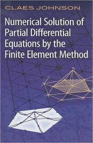
By Michael A. Golberg
Read Online or Download Numerical Solution of Integral Equations PDF
Best differential equations books
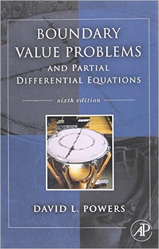
Boundary Value Problems: And Partial Differential Equations
Boundary price difficulties is the prime textual content on boundary worth difficulties and Fourier sequence for execs and scholars in engineering, technology, and arithmetic who paintings with partial differential equations. during this up to date variation, writer David Powers offers an intensive review of fixing boundary price difficulties concerning partial differential equations by way of the tools of separation of variables.
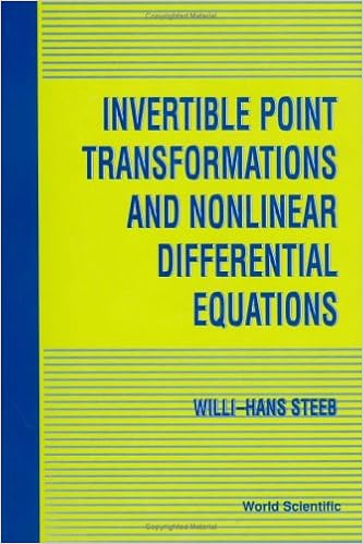
Invertible Point Transformations and Nonlinear Differential Equations
The invertible aspect transformation is a robust device within the research of nonlinear differential and distinction questions. This publication provides a finished creation to this method. usual and partial differential equations are studied with this strategy. The booklet additionally covers nonlinear distinction equations.
Dynamical systems and numerical analysis
This ebook unites the research of dynamical platforms and numerical answer of differential equations. the 1st 3 chapters comprise the weather of the speculation of dynamical structures and the numerical resolution of initial-value difficulties. within the last chapters, numerical tools are formulted as dynamical platforms and the convergence and balance homes of the tools are tested.
- Vorlesungen über Differenzenrechnung (Studien zur Sozialwissenschaft) (German Edition)
- An Introduction to Partial Differential Equations, 2nd edition, Edition: 2nd
- Principles of Partial Differential Equations (Problem Books in Mathematics)
- Elements of partial differential equations
- Elliptic Differential Equations and Obstacle Problems (University Series in Mathematics)
- Solution of Differential Equation Models by Polynomial Approximation (Physical & Chemical Engineering Science)
Additional resources for Numerical Solution of Integral Equations
Example text
Assume that the nonnegative function z (ξ) = −q (g(ξ))g (ξ) attains its positive maximum z (ξ M ) only at the point ξ M ∈ [a, b]. Then ts = min ξ∈[a,b] 1 1 = . 4 The method of characteristics revisited 39 Since xs belongs to the characteristics x = q (g (ξ M )) t + ξ M , we find xs = q (g (ξ M )) + ξM . 2. The point (xs , ts ) has an interesting geometrical meaning. 43) admits an envelope and (xs , ts ) is the point on the envelope with minimum time coordinate. 43) with respect to ξ. Clearly, the envelope has not to be confused with the shock curve.
We conclude this minimal introduction to finite difference approximation of scalar conservation laws by addressing some considerations about stability, which clarify the behavior of the approximate solution compared to the original model and represent a necessary requirement to make sure that the numerical approximation converges to the exact solution u. We briefly address the CFL condition (from Courant-Friedrichs-Lewy). It requires that the speed at which the scheme propagates the initial state must not be smaller than the characteristic speed of the model, namely |a| for the case ut +aux = 0.
7) we deduce ct = Dcxx − vcx which constitutes our mathematical model. 3 4 Assuming we can take the derivative inside the integral. [q] = [mass] × [time]−1 . 1. Notice that if v and D were non constant, we would get an equation of the form ct = (Dcx )x − (vc)x . 8). We want to determine the evolution of the concentration c, by knowing its initial profile c (x, 0) = g (x) . 9) can be written in the form vcx + ct = ∇c · v =0, pointing out the orthogonality of ∇c and v. But ∇c is orthogonal to the level lines of c, along which c is constant.