Metodos clasicos de resolucion de ecuaciones diferenciales by Varona, JL

By Varona, JL
Read or Download Metodos clasicos de resolucion de ecuaciones diferenciales ordinarias PDF
Best differential equations books
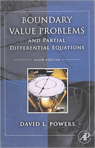
Boundary Value Problems: And Partial Differential Equations
Boundary price difficulties is the major textual content on boundary worth difficulties and Fourier sequence for execs and scholars in engineering, technology, and arithmetic who paintings with partial differential equations. during this up to date variation, writer David Powers presents a radical review of fixing boundary price difficulties regarding partial differential equations by way of the tools of separation of variables.
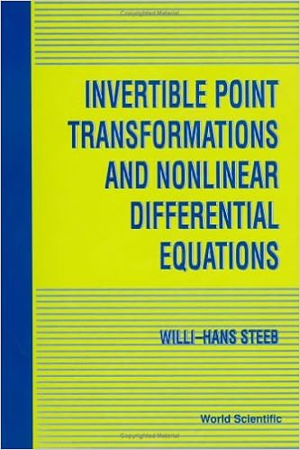
Invertible Point Transformations and Nonlinear Differential Equations
The invertible aspect transformation is a strong software within the examine of nonlinear differential and distinction questions. This ebook provides a finished creation to this method. traditional and partial differential equations are studied with this method. The publication additionally covers nonlinear distinction equations.
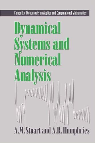
Dynamical systems and numerical analysis
This publication unites the learn of dynamical structures and numerical answer of differential equations. the 1st 3 chapters include the weather of the speculation of dynamical structures and the numerical answer of initial-value difficulties. within the final chapters, numerical tools are formulted as dynamical structures and the convergence and balance houses of the tools are tested.
- Partial differential relations
- Well-posed, Ill-posed, and Intermediate Problems with Applications (Inverse and Ill-Posed Problems)
- Differential Equations 3rd Edition Student Solutions Manual
- Well-posed, Ill-posed, and Intermediate Problems with Applications (Inverse and Ill-Posed Problems)
- Handbook of Differential Equations
Additional info for Metodos clasicos de resolucion de ecuaciones diferenciales ordinarias
Sample text
Log | cosec x − cotg x| + C = log tg sen x 2 (k) sh x dx = ch x + C. (l) ch x dx = sh x + C. (m) dx = th x + C. ch2 x (n) dx = − coth x + C. sh2 x (˜ n) 1 x 1 x dx = arc tg + C = − arc cotg + C1 , x2 + a 2 a a a a (o) (p) a > 0. x2 dx 1 x−a + C, = log 2 −a 2a x+a a2 1 1 x a+x dx + C = arg th + C, = log 2 −x 2a a−x a a + C. a = 0. a = 0. a = 0. (q) √ dx = log x + x2 + a x2 + a + C = 1 x arg sh √ + C, a a a > 0. (r) √ dx = log x + x2 − a x2 − a + C = 1 x arg ch √ + C, a a a > 0. (s) √ a2 x x dx = arc sen + C = − arc cos + C1 , 2 a a −x a > 0.
Cn−1 ) dx φ(x, C1 , . . , Cn−1 ) dx + Cn yn (x), donde Cn surge como constante de integraci´on al calcular una primitiva de φ (que aparece representada con la misma notaci´on de integral, esperando que este peque˜ no y habitual abuso de notaci´on no introduzca confusi´on en el lector). Si no conseguimos resolverla en general, se puede intentar reducir el orden de nuevo encontrando ahora un−1 (x) soluci´ on particular de la homog´enea asociada. Si este proceso lo logramos hacer el suficiente n´ umero de veces, llegaremos siempre a una ecuaci´on lineal de orden 1, que s´ı que sabemos resolver.
Lineal general de orden n > 1 no es soluble por cuadraturas. S´ı que pueden resolverse las ecuaciones lineales de orden n con coeficientes constantes; aunque ´este es un tema central en el estudio de la teor´ıa de E. D. , no nos ocuparemos de ello en estas notas. Realmente, lo u ´nico que vamos a ver aqu´ı es una serie de m´etodos que permiten reducir el orden de una E. D. Aplic´andolos (sucesivamente si es necesario), podremos llegar a una ecuaci´on de primer orden que, con un poco de suerte, se encontrar´a entre las que ya sabemos resolver.