Limit Cycles of Differential Equations by Colin Christopher
By Colin Christopher
This textbook includes the lecture sequence initially introduced on the "Advanced direction on restrict Cycles of Differential Equations" within the Centre de Rechercha Mathematica Barcelona in 2006. It covers the center-focus challenge for polynomial vector fields and the applying of abelian integrals to restrict cycle bifurcations. either issues are regarding the authors' pursuits in Hilbert's 16th challenge, yet might even be of curiosity to these operating extra in general within the qualitative idea of dynamical systems.
Read or Download Limit Cycles of Differential Equations PDF
Best differential equations books
Boundary Value Problems: And Partial Differential Equations
Boundary worth difficulties is the major textual content on boundary worth difficulties and Fourier sequence for pros and scholars in engineering, technology, and arithmetic who paintings with partial differential equations. during this up-to-date version, writer David Powers presents an intensive evaluation of fixing boundary worth difficulties regarding partial differential equations by means of the tools of separation of variables.
Invertible Point Transformations and Nonlinear Differential Equations
The invertible aspect transformation is a robust software within the examine of nonlinear differential and distinction questions. This e-book offers a accomplished advent to this system. traditional and partial differential equations are studied with this technique. The ebook additionally covers nonlinear distinction equations.
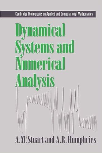
Dynamical systems and numerical analysis
This ebook unites the examine of dynamical platforms and numerical answer of differential equations. the 1st 3 chapters include the weather of the idea of dynamical platforms and the numerical answer of initial-value difficulties. within the last chapters, numerical tools are formulted as dynamical structures and the convergence and balance homes of the tools are tested.
- Advanced Engineering Mathematics with MATLAB, Fourth Edition (Advances in Applied Mathematics)
- Transport Equations in Biology (Frontiers in Mathematics)
- Differential Equations: LA Pietra 1996 : Conference on Differential Equations Marking the 70th Birthdays of Peter Lax and Louis Nirenberg, July 3-7, ... (Proceedings of Symposia in Pure Mathematics)
- Multilevel Adaptive Methods for Partial Differential Equations (Frontiers in Applied Mathematics)
Additional info for Limit Cycles of Differential Equations
Sample text
The generalized symmetry condition means that trajectories lying in x ≥ 0 can be mapped onto trajectories in x ≤ 0, with the points on x = 0 being fixed. If we know that the flow encircles the origin, then trajectories sufficiently close to the origin must be closed. Thus if the critical point is known to be of focal type, this generalized symmetry is enough to imply the existence of a center. 6, and consider h(x) = 2 A(x) − A(0) = x2 + O(x3 ). A (0) Clearly F and G are also polynomials of this polynomial, so that F = L(h(x)) and G = M (h(x)) for some polynomials L and M .
Cn are constants of k which are linearly independent over Q and u1 , . . un and v are in K. Then u1 , . . , un ∈ k and v = ct + d, with c a constant of k and d ∈ k. In our applications, we shall take k = C to ensure that k is algebraically closed. In particular, all elements of k are constants. The application we need of this result could probably be obtained by an application of complex variables, but we use the above result to emphasize the algebraic nature of the computations. We consider the system x˙ = y, y˙ = P0 (x) + P1 (x)y + P2 (x)y 2 .
3) has a non-degenerate center at the point x = p if and only g(p) = 0, g (p) > 0 and F and G are both polynomials of a polynomial A which satisfies A (p) = 0 with A (p) = 0. Proof. If we shift the x-axis to bring x = p to the origin, then it is clear that the new F and G calculated will differ from the original ones only by a constant. 6. 8. 3) into itself, reversing the directions. Thus the origin has a generalized symmetry. 3. 10) after a scaling. 3). Proof. 2. The generalized symmetry condition means that trajectories lying in x ≥ 0 can be mapped onto trajectories in x ≤ 0, with the points on x = 0 being fixed.