Elliptic Partial Differential Equations of Second Order, 2nd by David Gilbarg, Neil S. Trudinger

By David Gilbarg, Neil S. Trudinger
From the reviews:"This is a e-book of curiosity to any having to paintings with differential equations, both as a reference or as a e-book to profit from. The authors have taken difficulty to make the therapy self-contained. It (is) compatible required interpreting for a PhD scholar. even if the fabric has been built from lectures at Stanford, it has constructed into a nearly systematic insurance that's for much longer than can be lined in a year's lectures". e-newsletter, New Zealand Mathematical Society, 1985 "Primarily addressed to graduate scholars this based publication is obtainable and helpful to a extensive spectrum of utilized mathematicians". Revue Roumaine de Math?matiques Pures et Appliqu?es,1985
Read or Download Elliptic Partial Differential Equations of Second Order, 2nd edition PDF
Similar differential equations books
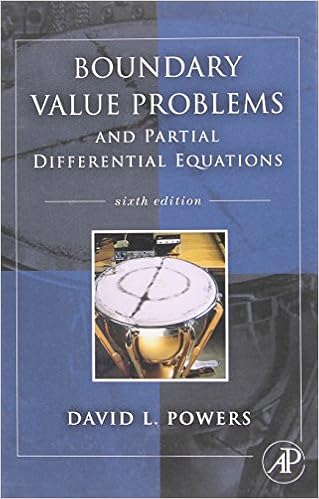
Boundary Value Problems: And Partial Differential Equations
Boundary worth difficulties is the major textual content on boundary price difficulties and Fourier sequence for execs and scholars in engineering, technological know-how, and arithmetic who paintings with partial differential equations. during this up-to-date version, writer David Powers offers a radical evaluate of fixing boundary price difficulties related to partial differential equations via the tools of separation of variables.
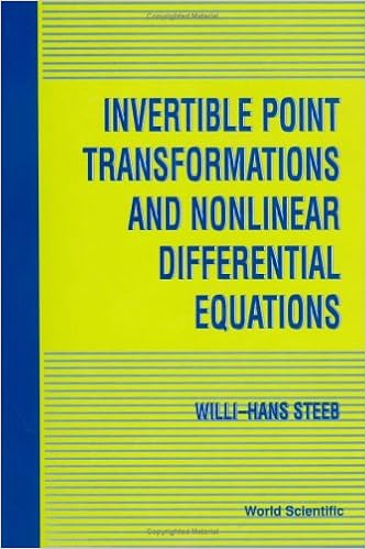
Invertible Point Transformations and Nonlinear Differential Equations
The invertible element transformation is a strong software within the examine of nonlinear differential and distinction questions. This publication provides a finished advent to this system. usual and partial differential equations are studied with this process. The ebook additionally covers nonlinear distinction equations.
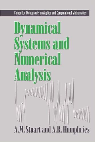
Dynamical systems and numerical analysis
This publication unites the examine of dynamical platforms and numerical answer of differential equations. the 1st 3 chapters include the weather of the speculation of dynamical platforms and the numerical resolution of initial-value difficulties. within the ultimate chapters, numerical equipment are formulted as dynamical platforms and the convergence and balance homes of the tools are tested.
- Lectures on algebraic solutions of hypergeometric differential equations (Lectures in mathematics)
- Spectral Representations for Schrödinger Operators with Long-Range Potentials (Lecture Notes in Mathematics)
- Differential Equations in Banach Spaces
- Handbook of Differential Equations - Evolutionary Equations
- Stochastic Integration and Differential Equations
Extra info for Elliptic Partial Differential Equations of Second Order, 2nd edition
Example text
40) by ′ E (u). 41) since E ′′ (u) 0 and ε > 0. 11 and integrate it over ΠT . Using the integrationby-parts formula, we transfer all the derivatives to the test function ϕ: u − ΠT f ′ (ξ )E ′ (ξ ) dξ dx dt ϕt E (u) + ϕx k ε ΠT ϕxx E (u) dx dt 49 The Kruzhkov lectures Passing to the limit as ε → +0, we get u ΠT f ′ (ξ )E ′ (ξ ) dξ dx dt ϕt E (u) + ϕx 0. 42) k Let {Em } be a sequence of C 2 -functions approximating the function u → |u − k| uniformly on R. 42) and pass to the limit ′ ′ as m → ∞. We can choose Em in such a way that Em is bounded and Em (ξ ) → sign(ξ − k ) for all ξ ∈ R, ξ = k .
7); this equality of the two areas is a direct consequence of the Rankine–Hugoniot condition. Figure 7. Area-preserving “overturning” of the graph. 7. 2). Denote +∞ S (t) = u(t, x) dx. , S (t) ≡ const. Proof. Indeed, we can write x(t) S (t) = +∞ u(t, x) dx + u(t, x) dx, x(t) −∞ where x = x(t) is the curve of discontinuity of the generalized solution u = u(t, x). As previously, we denote by u± = limx→x(t)±0 u(t, x) the one-sided limits (limits along the x-axis) of the solution u on the discontinuity curve.
Consequently, here the discontinuity is a weak, not a strong one. Now we can solve completely the Riemann problem for the Hopf equation. Here, two substantially different situations should be considered: (i) When u− > u+ , we can construct a shock wave solution, where the two constants u− and u+ are joined across the ray x = u2 +2 u1 t, according to the Rankine– Hugoniot condition (see Fig. 16): u(t, x) = u− for x < u+ for x > u− +u+ t, 2 u− +u+ t. 4) 52 Gregory A. Chechkin and Andrey Yu. Goritsky Figure 16.