Elementary matrices by Mitrinovic D.S.
By Mitrinovic D.S.
This educational textual content and challenge assortment is designed to introduce the scholar, at undergraduate or senior highschool point, to the ordinary houses of matrices and determinants. The advent offers a concise resume of undemanding matrix concept and the varied difficulties may still supply scholars a chance for vast perform in operating examples.
Read or Download Elementary matrices PDF
Best differential equations books
Boundary Value Problems: And Partial Differential Equations
Boundary worth difficulties is the best textual content on boundary price difficulties and Fourier sequence for execs and scholars in engineering, technological know-how, and arithmetic who paintings with partial differential equations. during this up-to-date version, writer David Powers presents a radical evaluation of fixing boundary price difficulties related to partial differential equations by means of the tools of separation of variables.
Invertible Point Transformations and Nonlinear Differential Equations
The invertible aspect transformation is a robust instrument within the research of nonlinear differential and distinction questions. This e-book offers a accomplished advent to this method. traditional and partial differential equations are studied with this procedure. The ebook additionally covers nonlinear distinction equations.
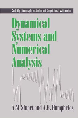
Dynamical systems and numerical analysis
This ebook unites the learn of dynamical platforms and numerical answer of differential equations. the 1st 3 chapters comprise the weather of the idea of dynamical platforms and the numerical resolution of initial-value difficulties. within the ultimate chapters, numerical equipment are formulted as dynamical platforms and the convergence and balance houses of the tools are tested.
- Ordinary Differential Equations in the Complex Domain (Dover Books on Mathematics)
- Hyperbolic Partial Differential Equations (Universitext)
- Multilevel Adaptive Methods for Partial Differential Equations (Frontiers in Applied Mathematics)
- Semiconcave Functions, Hamilton-Jacobi Equations, and Optimal Control (Progress in Nonlinear Differential Equations and Their Applications)
Additional info for Elementary matrices
Sample text
Rather than attempt to find the Γ, we reason as follows: eBt has entries eki\ Premultiphcation (multiplication on the left) by Γ"1 and postmultiplication (multiplication on the right) by T rearranges and combines these. 1) of the form [cYekit c2eXit y = _cne^_ [~ci] = eXitc, = eXtt _cn\ 5. THE CONSTANT COEFFICIENT CASE: REAL AND DISTINCT EIGENVALUES 31 where Af is one of the diagonal elements of B = TAT l. Then ~kiCie^~ = Ky, lfne kit or hy = Ay, which we write as (A - XJ)y = 0. 5). The (complex) numbers λ such that detG4-A/) = 0, are called the eigenvalues of the matrix A.
Given a sequence of matrices An, we can form another sequence (called the sequence of partial sums) by defining Sn = Ax + · · · + An. We denote the se quence {Sn} by £ " Ä 1 Ai and call J ^ Ai an infinite series. If limM_00 Sn = S, then the series is said to converge and its sum is defined to be S. If {Sn} does not converge, the series is said to diverge, and the sum is not defined. It is important to note that we can often show that a series converges without being able to find the limit. For example, we could investigate the (real) infinite series 00 νΠ o ni or the sequence of partial sums x2 xn and deduce that it converges.
Since all initial conditions can be satisfied, given a fundamental matrix 0,real solutions are of the form 0 ( t ) c , where 0 ( t )and c may have complex entries. Representing a real vector as the product of a matrix with complex entries and a constant vector with complex entries is, at least, inelegant and frequently may be awkward. For this reason we seek a way to find a real fundamental matrix. That this can always be done is a consequence of the following theorem. 6. 1). Proof. The complex-valued function φ(ί) can be written as q>(t) = u(t) + iv(t) where u(i) and v(t) are real-valued functions (u(t) = Re φ(ή, v(t) = lm