A concise course on stochastic partial differential by Claudia Prévôt
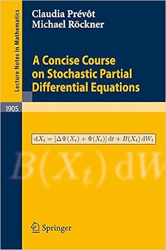
By Claudia Prévôt
These lectures pay attention to (nonlinear) stochastic partial differential equations (SPDE) of evolutionary variety. every kind of dynamics with stochastic impact in nature or man-made advanced structures will be modelled via such equations.
To retain the technicalities minimum we confine ourselves to the case the place the noise time period is given by means of a stochastic vital w.r.t. a cylindrical Wiener process.But all effects may be simply generalized to SPDE with extra normal noises equivalent to, for example, stochastic indispensable w.r.t. a continual neighborhood martingale.
There are primarily 3 methods to investigate SPDE: the "martingale degree approach", the "mild answer procedure" and the "variational approach". the aim of those notes is to provide a concise and as self-contained as attainable an advent to the "variational approach". a wide a part of invaluable historical past fabric, comparable to definitions and effects from the idea of Hilbert areas, are incorporated in appendices.
Read or Download A concise course on stochastic partial differential equations PDF
Best differential equations books
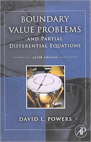
Boundary Value Problems: And Partial Differential Equations
Boundary worth difficulties is the prime textual content on boundary worth difficulties and Fourier sequence for pros and scholars in engineering, technology, and arithmetic who paintings with partial differential equations. during this up-to-date variation, writer David Powers presents a radical evaluate of fixing boundary worth difficulties related to partial differential equations by way of the equipment of separation of variables.

Invertible Point Transformations and Nonlinear Differential Equations
The invertible aspect transformation is a strong software within the research of nonlinear differential and distinction questions. This ebook provides a accomplished creation to this method. usual and partial differential equations are studied with this strategy. The booklet additionally covers nonlinear distinction equations.
Dynamical systems and numerical analysis
This ebook unites the examine of dynamical structures and numerical answer of differential equations. the 1st 3 chapters comprise the weather of the speculation of dynamical structures and the numerical answer of initial-value difficulties. within the closing chapters, numerical tools are formulted as dynamical platforms and the convergence and balance houses of the equipment are tested.
- Spectral and Dynamical Stability of Nonlinear Waves: 185 (Applied Mathematical Sciences)
- Differential Equations From The Algebraic Standpoint
- Differential Galois theory
- Partial Differential Equations III: The Cauchy Problem. Qualitative Theory of Partial Differential Equations (Encyclopaedia of Mathematical Sciences)
Additional resources for A concise course on stochastic partial differential equations
Example text
Let ek , k ∈ N, be an orthonormal basis of U0 = Q 2 (U ) and βk , k ∈ N, a family of independent real-valued Brownian motions. Define Q1 := JJ ∗ . 1) k=1 converges in M2T (U1 ) and defines a Q1 -Wiener process on U1 . e. J : U0 → Q12 U1 is an isometry. Proof. 1) is a Q1 Wiener process in U1 . If we set ξj (t) := βj (t)J(ej ), j ∈ N, we obtain that ξj (t), t ∈ [0, T ], is a continuous U1 -valued martingale with respect to Gt := σ σ(βj (s)|s t) , j∈N t ∈ [0, T ], since E(βj (t) | Gs ) = E(βj (t) | σ(βj (u)|u as σ σ(βj (u)|u s)) = βj (s) for all 0 s T∈[0,T ] Proof. 1) we may assume that sup |b(t, x)| |x| R Kt (R) for all R, t ∈ [0, ∞[. ) Fix R ∈ [0, ∞[ and define the (Ft )-stopping times τ (R, u) := inf{t 0|αt (R) > u}, u ∈ [0, ∞[. Since t → αt (R) is locally bounded, we have that τ (R, u) ↑ ∞ as u → ∞. In particular, there exists u(R) ∈ [0, ∞[ such that P ({τ (R, u(R)) R}) 1 . R 46 3. Stochastic Differential Equations in Finite Dimensions Setting τ (R) := τ (R, u(R)) we have τ (R) → ∞ in probability as R → ∞ and αt∧τ (R) (R) u(R) for all t, R ∈ [0, ∞[. Let (Wt )t 0 be a standard Wiener process on Rd1 , d1 ∈ N, with respect to Ft , t ∈ [0, ∞[. So, in the terminology of the previous section U := Rd1 , Q := I. The role of the Hilbert space H there will be taken by Rd , d ∈ N. Let M (d × d1 , R) denote the set of all real d × d1 -matrices. e. for each t their restriction to [0, t] × Ω is B([0, t])⊗Ft -measurable, for each fixed x ∈ Rd . We note that then both σ and b restricted to [0, t] × Rd × Ω are B([0, t]) ⊗ B(Rd ) ⊗ Ft -measurable for every t ∈ [0, ∞[.